Arranging the elements: the evolving design of the periodic table Inspire article
The periodic table hangs on the wall in just about every chemistry classroom. But its now-iconic design could have looked very different.
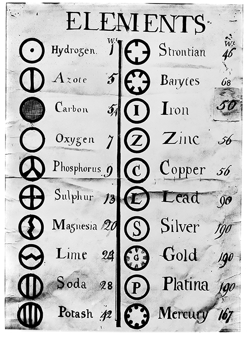
elements, showing the
symbols he had created for
each (click image to enlarge)
Wellcome Collection, CC BY 4.0
The credit for the creation of the periodic table generally goes to the chemist Dmitri Mendeleev. In 1869, he wrote out the known elements (of which there were 63 at the time) on cards and arranged them in columns and rows according to their chemical and physical properties.
But the periodic table didn’t actually start with Mendeleev. Many had tinkered with arranging the elements. Decades before, chemist John Dalton tried to create a table as well as some rather interesting symbols for the elements (figure 1), but they didn’t catch on. And just a few years before Mendeleev sat down with his deck of homemade cards, John Newlands created a table sorting the elements by their properties.
Mendeleev’s genius, however, was in what he left out of his table. He recognised that certain elements were missing, yet to be discovered. So where Dalton, Newlands and others had laid out what was known, Mendeleev left space for the unknown. Even more amazingly, he accurately predicted the properties of the missing elements.
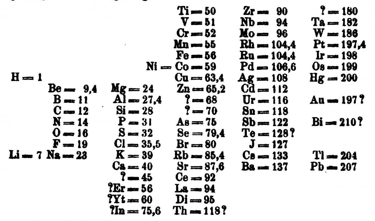
arrangement of the elements,
showing gaps for (then)
missing elements (click
image to enlarge)
Wikimedia Commons, public
domain
Notice the question marks in his table, shown in figure 2? For example, next to aluminium (Al), there is space for an unknown metal. Mendeleev foretold it would have an atomic mass of 68, a density of 6 g/cm3 and a very low melting point. Six years later, Paul Émile Lecoq de Boisbaudran isolated gallium and, sure enough, it slotted right into the gap with an atomic mass of 69.7, a density of 5.9 g/cm3 and a melting point so low that it becomes liquid in your hand. Mendeleev did the same for scandium, germanium and technetium (which wasn’t discovered until 1937, 30 years after his death).
At first glance, Mendeleev’s table doesn’t look much like the one we are familiar with. For one thing, the modern table has various elements that Mendeleev overlooked (and failed to leave room for), most notably the noble gases (such as helium, neon and argon). And the table is oriented differently to our modern version, with elements that we now place together in columns instead arranged in rows.
But once you give Mendeleev’s table a 90° turn, the similarity to the modern version (figure 3) becomes apparent. For example, the halogens – fluorine (F), chlorine (Cl), bromine (Br) and iodine (I) (the J symbol in Mendeleev’s table in figure 2) – all appear next to one another. Today, they are arranged in the table’s 17th column.
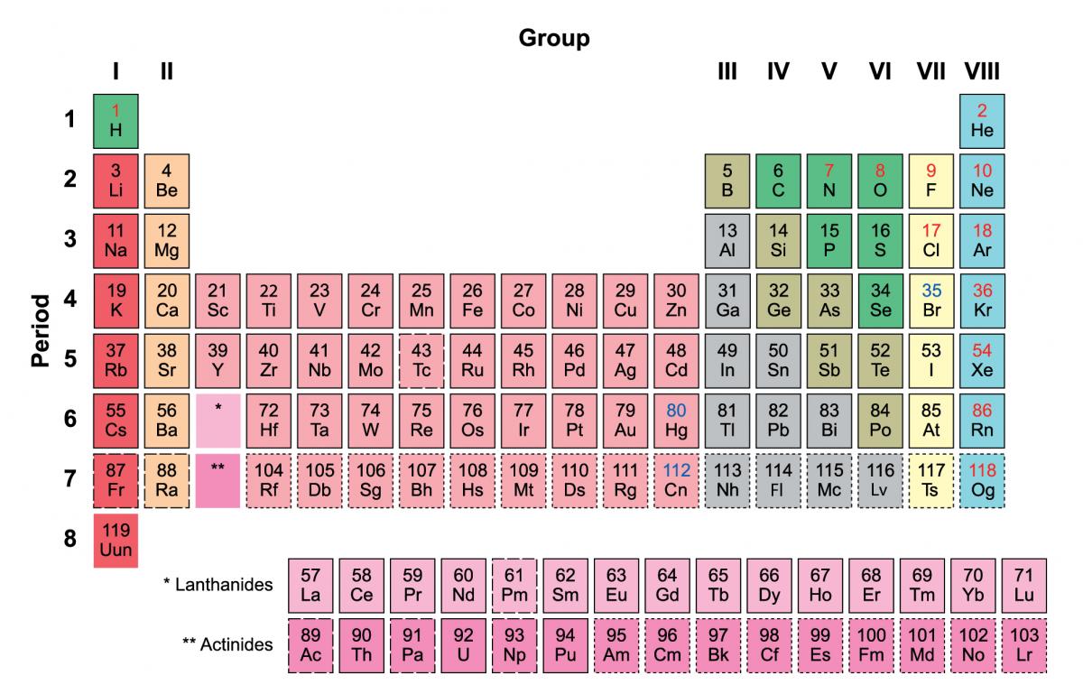
Armtuk/Wikimedia Commons, CC BY-SA 3.0
Period of experimentation
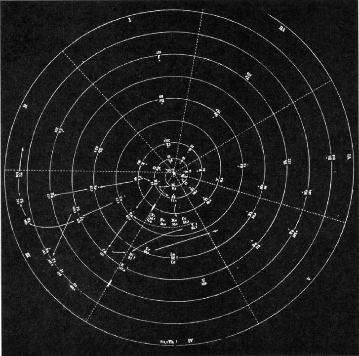
spiral arrangement of the
elements, with hydrogen at
its centre. Reprinted with
permission from Quam &
Quam (1934) (click image to enlarge)
Copyright Division of Chemical
Education, Inc. of the American
Chemical Society
It may seem a small leap from this to the familiar diagram but, years after Mendeleev’s publications, there was plenty of experimentation with alternative layouts for the elements. Even before the table got its permanent right-angle flip, some weird and wonderful twists had been suggested.
One particularly striking example is Heinrich Baumhauer’s spiral (figure 4), published in 1870, with hydrogen at its centre and elements with increasing atomic mass spiralling outwards. The elements that fall on each of the wheel’s spokes share common properties – just as those in a group do so in today’s table. There was also Henry Basset’s rather odd ‘dumbbell’ formulation of 1892.
Nevertheless, by the beginning of the 20th century, the table had settled down into a familiar horizontal format, with a modern-looking version from Alfred Werner in 1905. For the first time, the noble gases appeared in their now-familiar position at the far right of the table. Werner also tried to take a leaf out of Mendeleev’s book by leaving gaps, although he somewhat overdid the guesswork with suggestions for elements lighter than hydrogen and another sitting between hydrogen and helium – none of which exist.
Despite Werner’s progress, there was still a bit of rearranging to be done. Particularly influential was Charles Janet’s version in 1929 (figure 5). He took a physicist’s approach to the table and used the newly discovered quantum theory to create a layout based on electron configurations. The resulting ‘left step’ table is still preferred by many physicists. Interestingly, Janet also provided space for elements right up to number 120, despite only 92 being known at the time (we’re only at 118 now).
Wikipedia, CC BY-SA
Settling on a design
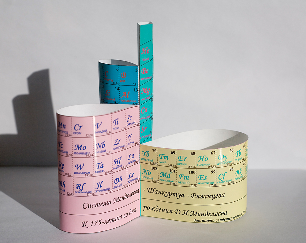
flower’ version of the periodic table
(click image to enlarge)
Тимохова Ольга/Wikimedia
Commons, CC BY-SA 3.0
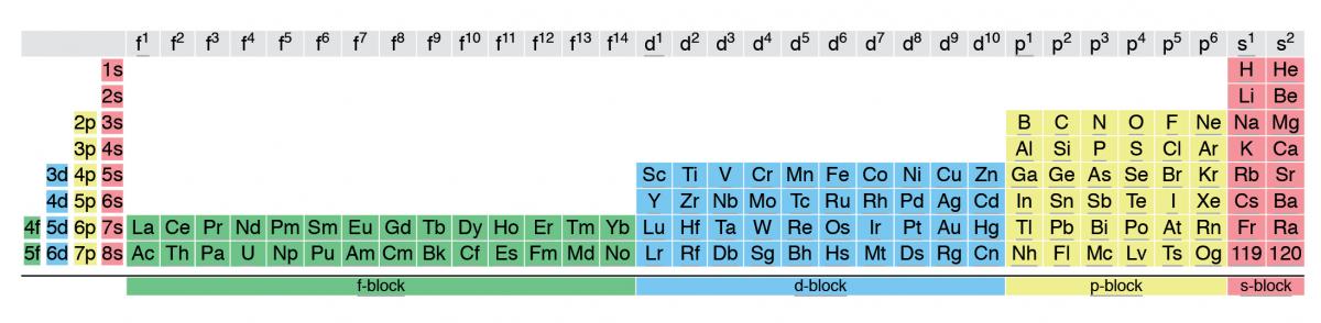
The modern table is actually a direct evolution of Janet’s version. The alkali metals (the group topped by lithium) and the alkaline earth metals (topped by beryllium) were shifted from the far right to the far left to create a very wide-looking (long-form) periodic table. The problem with this format is that it doesn’t fit nicely on a page or poster, so, largely for aesthetic reasons, the f-block elements are usually cut out and deposited below the main table. That’s how we arrived at the table we recognise today.
That’s not to say that people haven’t continued to tinker with its design, often as an attempt to highlight correlations between elements that aren’t readily apparent in the conventional table. There are literally hundreds of variationsw1, with spirals and 3D versions (figure 6) being particularly popular, not to mention more playful variants.
How about my own fusion of two graphics: Mendeleev’s table and Henry Beck’s London Underground map (figure 7)? Or the dizzy array of lookalike ‘periodic tables’ categorising everything from beer to Disney characters – all of which go to show how the periodic table of elements has become the iconic symbol of science.
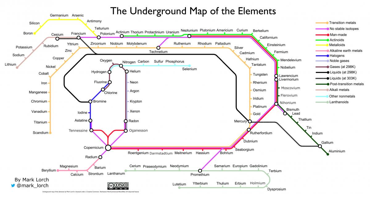
Mark Lorch, CC BY NC-SA 3.0
Acknowledgement
This is an edited version of an article originally published on The Conversation UK. Read the original article at The Conversation UK websitew2.![]()
References
- Quam GN, Quam MB (1934) Types of graphic classifications of the elements. III. Spiral, helical, and miscellaneous charts. Journal of Chemical Education 11: 288-297. doi: 10.1021/ed011p288
Web References
- w1 – Explore hundreds of iterations of the periodic table at Mark Leach’s database.
- w2 – The Conversation is an independent source of news and opinions written by academics and researchers for the public. To see the original version of this article, visit The Conversation UK website.
Resources
- Listen to Tom Lehrer’s song ‘The Elements’ about the periodic table.
- Watch a video of the gallium ‘beating heart’ experiment from the University of Nottingham’s Periodic Table of Videos series.
- Find out about some of the less celebrated scientists, many of them women, who contributed to the development of the periodic table. See:
- Lykknes A, Van Tiggelen B (2019) In their element: women of the periodic table. Science in School 47: 8-13.